What the plot shows
The horizontal axis is dimensionless position $x$. The vertical
axis is energy: $V(x)$ and $E$ share the labelled scale on the
left. The wavefunction overlays — bright $|\psi|^2$ envelope and
faint $\mathrm{Re}\,\psi$ oscillation — are auto-scaled to fit the
same panel, so their visual amplitude is not in
the same units as the energy ticks. Treat them as a shape, not a
magnitude comparison against $V$.
- Shaded grey region: $V(x)$, the potential.
- Dashed green line: the chosen energy $E$.
- Bright white curve: $|\psi(x)|^2$, the probability density.
- Faint grey curve: $\mathrm{Re}\,\psi(x)$, exposing the local wavelength.
All potentials are non-negative, so $V$ never goes
below the energy axis. For the well, $V_0$ is the height of the
surrounding walls and the well floor sits at $V = 0$.
The equation being solved
We solve the time-independent Schrödinger equation in one dimension:
$$ -\frac{\hbar^2}{2m}\, \psi''(x) \;+\; V(x)\, \psi(x) \;=\; E\, \psi(x) $$
Setting $\hbar = m = 1$ reduces this to:
$$ \psi''(x) \;=\; 2\,\big(V(x) - E\big)\, \psi(x) $$
Where $E > V$ the right-hand side is negative and $\psi$ oscillates
with local wavenumber $k(x) = \sqrt{2(E - V(x))}$. Where $E < V$ the
right-hand side is positive and $\psi$ grows or decays exponentially
at rate $\kappa(x) = \sqrt{2(V(x) - E)}$. The equation is integrated
as one continuous ODE — there is no separate region matching, so
continuity of $\psi$ and $\psi'$ across a step in $V$ is automatic.
Potentials available
- Barrier: $V(x) = V_0$ for $|x| < w/2$, else $0$.
- Well: $V(x) = 0$ for $|x| < w/2$, else $V_0$ (free region between walls).
- Step: $V(x) = V_0 \cdot \Theta(x)$.
- Double: two barriers of height $V_0$ separated by a gap; supports resonant tunneling.
- Gaussian: $V(x) = V_0 \exp\!\left(-x^2 / 2\sigma^2\right)$, $\sigma = w / 2.355$.
All sharp edges are replaced by $\tanh$ transitions of width
$\varepsilon = 0.04$ — about one grid spacing. Visually the edges
still look sharp, but the integrator sees a continuous $V(x)$ and
its fourth-order accuracy is preserved.
Boundary conditions and how they are enforced
Scattering boundary conditions: incoming plane wave from the left of
unit amplitude, reflected wave of amplitude $r$, transmitted wave on
the right of amplitude $t$, and no incoming wave
from the right.
$$ \psi(x \to -\infty) = e^{i k_L x} + r\, e^{-i k_L x} $$
$$ \psi(x \to +\infty) = t\, e^{i k_R x} $$
where $k_L = \sqrt{2(E - V_L)}$ and $k_R = \sqrt{2(E - V_R)}$, and
$V_L, V_R$ are the asymptotic values of $V$. For barrier, double
and Gaussian, $V_L = V_R = 0$, so $k_L = k_R = \sqrt{2E}$. For the
well, $V_L = V_R = V_0$ and the wave is only propagating on the
outside if $E > V_0$. For the step, $V_L = 0, V_R = V_0$.
The right boundary is enforced by construction. We
start integration at $x = +L$ with $\psi = e^{i k_R x}$ and
$\psi' = i k_R e^{i k_R x}$. There is no left-moving component to
remove because we never put one in. When $E < V_R$ there is no
propagating outgoing wave — we instead start with the decaying
$\psi = e^{-\kappa_R x}$.
The left boundary is enforced by decomposition.
After integration reaches $x = -L$ the solution is a superposition
$A\, e^{i k_L x} + B\, e^{-i k_L x}$. Solving for $A, B$ from
$\psi(-L)$ and $\psi'(-L)$:
$$ A = \tfrac{1}{2}\, e^{-i k_L L}\, \big(\psi - i\, \psi' / k_L\big) $$
$$ B = \tfrac{1}{2}\, e^{+i k_L L}\, \big(\psi + i\, \psi' / k_L\big) $$
Physical normalization sets the incoming amplitude to $1$, which
means dividing every amplitude by $A$: so $t = 1/A$ and $r = B/A$.
When $E < V_L$ there is no propagating wave on the left at all —
the asymptotic region is classically forbidden and an "incoming
plane wave" does not exist. The simulator detects this case and
shows a sub-threshold notice on the plot; $T$ is set to $0$ and the
rendered $\psi$ is just the right-boundary solution propagated
left, normalized to its own peak (it is not a physical scattering
state in this regime).
Probability and normalization
Scattering states are not square-integrable — $\int |\psi|^2\, dx$
diverges because the asymptotic plane waves never decay. The
normalization convention is therefore fixed incoming
amplitude, not unit total probability. With incoming
amplitude $1$:
- On the left: $|\psi|^2 = \big|1 + r\, e^{-2 i k_L x}\big|^2$, oscillating between $(1 - |r|)^2$ and $(1 + |r|)^2$ due to standing-wave interference.
- On the right: $|\psi|^2 = |t|^2$, constant.
The conserved quantity is the probability current,
not the density. Current conservation gives:
$$ T + R = 1, \qquad T = \frac{k_R}{k_L}\, |t|^2, \qquad R = |r|^2 $$
The factor $k_R / k_L$ matters for the step potential where
$k_R \neq k_L$; otherwise it equals $1$. The reported $T$ and $R$
always sum to $1$ to numerical precision — drift from $1$ is a
useful sanity check on the integrator. When $E < V_R$ the right
side is evanescent, so $T = 0$ and $R = 1$ exactly.
Algorithm
The full pipeline runs on every slider input event:
- Pick a domain $[-L, L]$ with $L = \max(15,\, 4w + 4)$, so the boundaries sit comfortably outside the potential. Discretize into $N = 1200$ uniform points.
- Sample $V(x_i)$ on the grid using the $\tanh$-smoothed shape definitions.
- Compute $k_L, k_R$ (or $\kappa_L, \kappa_R$) from the boundary potentials and the current energy.
- Initialize the state at $x = +L$ with the outgoing-only boundary form (or the decaying form if $E < V_R$).
- Integrate the second-order ODE backward to $x = -L$ using classical fourth-order Runge–Kutta on the first-order system $y = (\mathrm{Re}\,\psi,\, \mathrm{Im}\,\psi,\, \mathrm{Re}\,\psi',\, \mathrm{Im}\,\psi')$.
- If $E > V_L$: decompose $\psi(-L), \psi'(-L)$ into $A, B$. Otherwise mark sub-threshold.
- Compute $T = (k_R / k_L)\, |1 / A|^2$ and $R = |B / A|^2$.
- Rescale every $\psi(x_i)$ by $1/A$ so the incoming amplitude becomes $1$, then render on canvas.
Why integrate backward? Forward shooting from the
left would require guessing both $r$ and $t$ and enforcing the
no-incoming-from-right condition at $+L$ by iteration. Backward
shooting collapses that to a single pass: the right boundary is a
known initial condition (one outgoing plane wave), and the unknowns
$r, t$ drop out of a linear decomposition at the left.
Verification
Spot-checks against the textbook closed forms:
- Step up ($E = 15$, $V_0 = 8$): analytical $T = 4 k_L k_R / (k_L + k_R)^2 \approx 0.964$; simulator returns $0.968$.
- Step under ($E = 5$, $V_0 = 8$): analytical $T = 0$, $R = 1$ exactly; simulator matches.
- Rectangular barrier ($E < V_0$): exponentially small $T \approx \exp(-2 \kappa w)$; simulator matches the order of magnitude.
- Finite-walls well ($E > V_0$): transmission resonances at $k\, w_{\text{free}} = n\pi$; visible as $T = 1$ peaks when sweeping $E$.
Residuals are sub-percent, dominated by the smoothing of $V$
discontinuities. Increasing $N$ or decreasing $\varepsilon$ closes
the gap at the cost of redraw time.
Where this falls short
- Strictly steady-state scattering, not a wavepacket movie. The plot is the eigenstate of the scattering Hamiltonian at the chosen $E$.
- Probability density on the left interferes with the reflected wave and oscillates between roughly $0$ and $4$ for total reflection. Physical, not an integrator artifact.
- Very narrow resonance peaks (thin gap in the double barrier with a tall $V_0$) can be skipped by the slider's discrete steps. Drag slowly through likely resonance regions.
- For very large $V_0 w$ the unnormalized $|A|^2$ can grow large enough to lose precision; the UI clamps $T, R$ to $[0, 1]$.
- The well's bound-state eigenvalues (when $E < V_0$) are not solved here — that is an eigenvalue problem, not scattering.